Sampling from a multivariate discrete distribution

Generating random samples is a key step in Monte Carlo simulations. Examples are computing the expectation or the variance of a random variable, estimating quantiles (and synthesising fancy, realistic images as pursuit by many people these days). In this post we consider sampling from discrete distributions, namely those defined on sets of finite elements. In a nutshell, this post is about approximating a (unnormalised) distribution with a tractable one, a common setting in Bayesian inference.

Introduction

Let us define some symbols:

• \(\mathcal{X}=\{0,\dots, L-1\}^D\): a finite lattice, where \(D \geq 1\) and \(L>1\),
• \(p\): a probability mass function (pmf) on \(\mathcal{X}\); \(p(x) > 0\) everywhere.

Our goal in this post is to sample from the distribution \(p\) on \(\mathcal{X}\). An example of such distributions is the Ising model, where there are \(D\) lattice sites taking binary states (\(L=2\)).

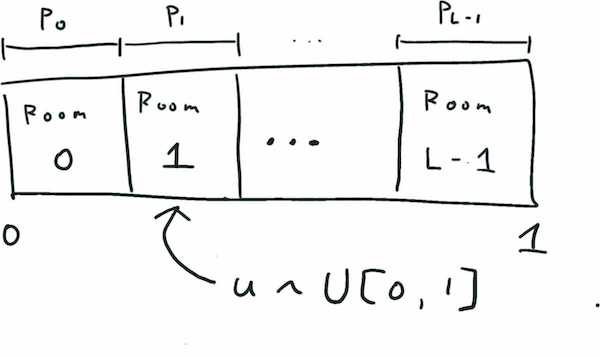
How do we approach this? Let us first consider the simple case \(D=1\). In this case, we can sample from the distribution using the inverse trick. The crux is that a probability distribution defines a partition of the unit interval. If we draw a sample from the uniform distribution \(U[0,1]\) on the interval, then the probability of falling in a room, say Room 1, is the length of the room, which is \(p(1)\).

This approach in theory can be extended to \(D>1\) by noting that a probability distribution defines a partition of the unit cube; however practically, this is no longer tractable in high dimension:

1. Computing the partition of the unit cube is expensive in time (note that the cardinality of \(\mathcal{X}\) is \(L^D\)), and
2. Even if we get the partition, we cannot (at least naively) store it in memory.

Clearly, we need alternatives. But what else can we do? Here, we simply consider approximating the distribution \(p\) with a tractable one \(q\) from which we can generate samples.

Sampling with approximate distributions

An obvious problem with approximation is that we do not have many options for \(q\); if \(q\) is too complicated, then we face the same intractability issue. Anyway let’s first consider a simple approach. A first candidate is coordinate-wise independent distributions, that is, in the form of

\[\begin{equation} q(x^1, \dots, x^D) = \prod_{d=1}^Dq^{(d)}(x^d), \tag{prod}\label{product} \end{equation}\]

where \(q^{(d)}:\{0,\dots, L-1\} \to [0,1]\), \(d=1,\dots,D\). Let us call a distribution of the above form a rank-one distribution.

We know that for one-dimensional distributions, sampling is trivial. The independence structure in the above form makes sampling efficient, as we only need to sample each coordinate variable \(x^d\) independently (so the cost is \(O(LD)\) if it is done sequentially). While this is a huge improvement from \(O(L^D)\), a drawback of this approximate family is that it completely ignores interactions among coordinate variables \(x^d\) that might be present in \(p\). For instance, if \(p\) represents a distribution of text sequences, then ignoring dependencies means that the approximant disregards certain cooccurence of words.

Unfortunately, we cannot just improve the expressiveness of the family by introducing complex interactions to \(q\) – sampling is again difficult. So, is this the end of the post? Of course, no. A kind of standard approach to extend such simple distributions is to take mixtures, like we do with Gaussian mixtures. Why is this an okay approach? To see this, let us treat \(p\) as a probability tensor (or an array) with \(D\) indices. Then, \(p\) can be written as a mixture of rank-one tensors:

\[\begin{align} &p(x^1=i_1, \dots ,x^D=i_D)\\ &= p(x^1=i_1|x^2=i_2,\dots,x^D=i_D)p(x^2=i_2,\dots,x^D=i_D)\\ &= \sum_{j_2}^L\cdots\sum_{j_D=1}^L p(x^2=i_2,\dots,x^D=i_D) \underbrace{p(x^1=i_1|x^2=i_2,\dots,x^D=i_D) \delta_{i_2, j_2} \cdot \cdots \cdot \delta_{i_D, j_D}}_{a_{i_1,j_2,\dots,j_D}} \end{align}\]

where \(\delta\) is the Kronecker delta; \(a=p(x_1=\cdot|i_2,\dots,i_D)\otimes e_{i_2}\otimes \cdots \otimes e_{i_D}\) with the symbol \(\otimes\) denoting the outer product of vectors, and \(e_{i_j}\) denotes the standard basis vector. The tensor product \(p(x_1=\cdot|i_2,\dots,i_D)\otimes e_{i_2}\otimes \cdots \otimes e_{i_D}\) is a rank-one distribution where all but the first coordinates put all their mass on particular symbols in \(\{0, \dots, L-1\}\). While this example is somewhat vacuous, it at least shows that the any distribution has some low-rank decomposition, justifying the approximation.

If you have experience in tensor decomposition, you have probably noticed that the above mixture distribution is an instance of Canonical Polyadic (CP)-decomposition

\[\begin{align} p = \sum_{r=1}^R \lambda_r \cdot q_r^{(1)} \otimes \cdots \otimes q_r^{(D)}. \end{align}\]

In general, we can consider the following form of mixture models:

\[\begin{equation} q_{\mathrm{mix}} = \int (q^{(1)} \otimes \cdots \otimes q^{(D)}) \mathrm{d}Q(q^{(1)}, \dots, q^{(D)}), \tag{mixture}\label{mixture} \end{equation}\]

where \(Q\) is a joint distribution of probability vectors \(q^{(1)},\dots, q^{(D)}\) (so the above expression is simply averaging with respect to the distribution \(Q\)). Sampling from \(q_{\mathrm{mix}}\) is straightforward by ancestral sampling, which is performed as follows

1. Sample \((q^{(1)},\dots, q^{(D)}) \sim Q.\)
2. Sample \((x^1,\dots,x^D) \sim q^{(1)}\otimes \dots \otimes q^{(D)}.\)

Note that a CP-decomposition corresponds to setting the mixing distribution \(Q\) to a mixture of Dirac deltas

\[Q_{\mathrm{CP}} = \sum_{r=1}^R \lambda_r \delta_{q_r^{(1)} \otimes \cdots \otimes q_r^{(D)}},\]

where each \(\delta_{q_r^{(1)} \otimes \cdots \otimes q_r^{(D)}}\) corresponds to a fixed rank-one distribution. As a side note, we mention that the family \(q_{\mathrm{mix}}\) also includes the Tucker-decomposition as we can choose

\[Q_{\mathrm{Tucker}} = \sum_{r_1=1}^{R_1}\cdots \sum_{r_D=1}^{R_D}c_{r_1,\dots,r_D}\delta_{q_{r_1}^{(1)} \otimes \cdots \otimes q_{r_D}^{(D)}},\]

where \(c\) is a probability tensor (of size typically smaller than \(p\)). While the infinite mixture looks like an overkill, we will make use of this flexible form to learn approximations rather than turn to low-rank tensor decompositions.

Another family of flexible distributions is auto-regressive models (like huge transformer models). Although it can be used in our following discussion, we will focus on the above mixture model for simplicity.

Learning approximate distributions

In the following, we consider a concrete approach to construct an appropriate

\[q = \int (q^{(1)} \otimes \cdots \otimes q^{(D)}) \mathrm{d}Q(q^{(1)}, \dots, q^{(D)}).\]

Mixing distribution

Perhaps not surprisingly, we can use neural network to construct a mixing distribution \(Q\). Let

\[f_{\theta}: \mathbb{R}^{D_z}\to \mathbb{R}^{\underbrace{L\times\cdots\times L}_{D \text{ times}}}\]

be a neural network. We define a distribution \(Q_{\theta}\) by the following generative process:

1. Draw a noise vector \(z\) from some distribution on \(\mathbb{R}^{D_z}\) (e.g., Gaussian).
2. Convert \(z\) by feeding to \(f_{\theta}\); obtain \((q^{(1)},\dots,q^{(D)})=\tilde{f}_{\theta}(z)\),

where \(\tilde{f}_{\theta}\) is the normalised version of \(f_{\theta}\). (Thus we define \(Q_{\theta}\) as a push-forward given by \(\tilde{f}_{\theta}.\))

Training objective – kernel Stein discrepancy

Now that we have defined a concrete model class \(Q_{\theta}\), we want to optimise the parameter \(\theta\) so that the resulting \(q_{\mathrm{mix}}\) is close to \(p\). This demands a discrepancy measure that tell us how good our approximation is; It is required that the discrepancy can be estimated using (a) evaluation of \(p\) and (b) samples from \(q_{\mathrm{mix}}\). Note that the pmf of the approximant \(q_{\mathrm{mix}}\) is not given in closed form due to the complicated mixing distribution \(Q_{\theta}\), which is why we can only assume access to generated samples. As a consequence, common discrepancy measures such as KL-divergence are ruled out.

As the heading suggests, we use the kernel Stein discrepancy (KSD) (Yang et al., 2018). KSD is defined by two ingredients: a score function and a kernel. The score function of a pmf \(p\) is defined as follows¹:

\[\mathbf{s}_p(x) = {1 \over p(x)}\cdot (\Delta^1 p(x), \dots, \Delta^D p(x)),\]

where \(\Delta^i\) denotes taking a forward-difference (mod \(L\)) w.r.t. the \(i\)-th coordinate

\[\Delta^i p(x) = p(x^1,\dots,\bar{x}^i,\dots,x^D) - p(x^1,\dots,x^i,\dots,x^D),\ \bar{x}^i = x^i + 1\text{ mod } L.\]

Note that if \(p\) is given by normalising a function \(g\), i.e., \(p(x) = g(x)/Z\), the score function does not depend on the normalising constant \(Z\). A kernel function \(k:\mathcal{X}\times \mathcal{X}\to \mathbb{R}\) is simply a positive definite kernel.

Based on these items, the (squared) KSD is defined as

\[\mathrm{KSD}^2_p(q) = \mathbb{E}_{x\sim q}\mathbb{E}_{x'\sim q}[h_p(x,x')],\]

where \(h_p\) is a function defined by

\[\begin{equation} \begin{aligned} h_p(x,x') &= \mathbf{s}_p(x)^{\top} \mathbf{s}_p(x') k(x,x') + \mathbf{s}_p(x)^{\top} \Delta^*_{x'} k(x, x')\\ &\quad +\mathbf{s}_p(x')^{\top} \Delta^*_x k(x, x') + \mathrm{tr} \Delta_x^*\Delta_{x'}^*k(x,x'). \end{aligned} \tag{stein kernel}\label{skernel} \end{equation}\]

Here, \(\Delta_x^*\) is the inverse difference operator defined as for \(\Delta\) that acts on \(x\) such that

\[\begin{align} &\Delta^{*}_{x} k(x, x') = \bigl(k(x, x') - k(x^1, \dots, \tilde{x}^i, \dots, x^D,x')\bigr)_{i=1}^D,\\ & \text{where }\tilde{x}^i = x^i - 1 \text{ mod } L.\\ \end{align}\]

The KSD is a valid discrepancy measure: \(\mathrm{KSD}_p(q)=0\) if and only if \(p=q\). Given sample points \(\{x_i\}_{i=1}^n\) from \(q\), the KSD can be easily estimated with

\[\widehat{\mathrm{KSD}^2}_p(q) = {1\over B}\sum_{b=1}^B h(x_{i_b}, x_{j_b}), \tag{ksdest}\label{ksdest}\]

where the indices \(1\leq i_b < j_b \leq n\) are sampled uniformly from all possible pairs, and \(B\) is a batch-size \((1 \leq B \leq n(n-1)/2)\).

Training specifics – differentiability

You might have wondered if the training objective \(\widehat{\mathrm{KSD}^2}_p(q)\) in (\ref{ksdest}) is differentiable or not. First of all, the forward/backward difference operations in (\ref{skernel}) can be performed with matrix multiplications as shift operations are permutations (in one-hot encoding). Second, the discrete nature of samples \(\{x_i\}_{i=1}^n\) from \(q\) does not allow us to do gradient-based learning. Fortunately, by continuous relaxation, we can circumvent this issue – there is a well-known trick called the Gumbel-softmax trick (Jang et al., 2016, Maddison et al., 2016). Specifically, to sample a continuously relaxed version of \((x^1,\dots, x^D) \sim q^1\otimes \dots \otimes q^D\), we only need to sample \(D\) independent samples \((u^d)_{d=1}^D\) from the Gumbel distribution \(G(0, 1)\), and for each \(d\), take \(\mathrm{softmax}\Bigl([q^d + u^d]/\tau\Bigr)\) with a temperature parameter \(\tau>0\). Note that because of this sampling method, the normalisation of \(f_{\theta}(z)\) is not necessary. For details, see the papers Jang et al., 2016, Maddison et al., 2016. Therefore, the model \(q\) defined by the distribution \(Q_{\theta}\) can be learned with back propagation and implemented straightforwardly in e.g., PyTorch. Lastly, a kernel function such as the Gaussian kernel that acts on one-hot vectors can be used.

So, is it good…?

Unfortunately, I cannot give you a definite answer in this post. I compared the mixture model (\ref{mixture}) with the product of categoricals in (\ref{product}) on an energy-based model

\[p(x) \propto \exp(\mathrm{NN}(x))\]

for some neural network \(\mathrm{NN}\) that does not necessarily have a sparse (or low-rank) structure. For this task, I observed that (somewhat obviously) the mixture model has a better performance in terms of KSD than the product one (see the plot below). The ipynb for this experiment is here.

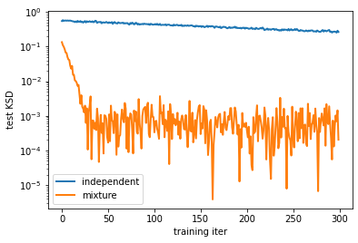
Evaluating the goodness of an approximation is a somewhat delicate issue. For example, a low KSD value might not be aligned to the quality of generated images if \(p\) represents a distribution on images; we might want \(q\) to capture (some order of ) moments of \(p\), and it would be desirable that KSD could indicate if \(q\) is a good approximation in this sense. The training of the network might get stuck in some bad optima, or the network might be optimised to capture some trivial features of \(p\). My evaluation is not thorough, but the result at least hints that \(q\) has some potential (compared to the vanilla choice (\ref{product})).

End remarks

The use of Stein discrepancies in variational inference has been proposed in Ranganath et al., 2016. A theoretical understanding of learning a posterior approximation with KSD has been established by Fisher et al., 2020, where the approximating distribution is defined by measure transport. In the discrete case, defining a push-forward of some continuous distribution to a discrete distribution is not so trivial, and therefore we considered a mixture model where the density (pmf) is explicitly given. On a related note, a discrete version of normalizing flows have been considered in Tran et al., 2019.

Variational inference with a mixture model like in (\ref{mixture}) is known as semi-implicit variational inference (see, e.g., Yin and Zhou, 2018). I am sure that there have been significant developments in this area. A relative benefit of using KSD is that we can directly optimise w.r.t. a discrepancy measure (rather than a lower bound of marginal likelihood).